Digital Filter
A digital process by which an input is processed to yield a desired output; filter output requirements are often specified in terms of frequency domain parameters.
Impulse Response
The output of a digital (or analog) filter when given a short "burst" input. This impulse input, typically denoted h(n) (or h(t) for the analog counterpart), has a magnitude of 1 when n = 0 (or at time T = 0), and has a magnitude of 0 thereafter. The output rendered by the filter after n = 0 (or time T = 0) is characteristic of the filter itself, and is a relatively accurate way of mathematically describing the filter response. The magnitude of the impulse response of a filter will eventually decay to 0.
FIR Filter
The magnitude of a Finite Impulse Response digital filter will decay to 0 after a finite number of sample periods when subjected to an impulse input. An FIR filter uses only present and past inputs when implemented, is always stable, and exhibits linear phase throughout its frequency response. An FIR filter, however, will require a higher order to achieve the same band-limiting and cutoff transition zone width in its frequency response as its IIR counterpart.
IIR Filter
The magnitude of an Infinite Impulse Response digital filter will decay to 0 only as n number of sample periods goes to infinity. An IIR filter uses present and past outputs as well as present and past inputs, can become unstable if not properly designed and implemented, and exhibits non-linear phase throughout its frequency response. An IIR filter is generally more efficient in terms of band-limiting in its frequency response than a FIR filter of the same order.
Sample Period
Time period between consecutive digital captures of an analog input signal, or between consecutive digital bias-levels of a digital output signal.
Sample Frequency
1 / Sample Period
Nyquist Frequency
1/2 of the Sample Frequency; aliasing will occur above this frequency.
Aliasing
The apparent repetition or "folding" of frequencies below the Nyquist frequency to the range above the Nyquist frequency; a soprano singer who has a tone which is higher than the Nyquist frequency at which she is recorded will likely sound like a baritone when the recording is played back.
Z Operator
The Z Transform is a basic tool in the realm of DSP. The delay operator "Z" is derived from the Laplace delay model used in the differential equation representation of signals and systems.
If one desires to design in the Laplace domain and transform into the Z domain, solving for S requires manipulation of the natural log. Approximations make use of representing the natural log with various forms of a truncated infinite power series. Two useful results are the "Backward-Difference" and "Bilinear" transformations.
The backward-difference transformation maps lower frequencies from the S-domain to the Z-domain reasonably well, but is not as successful as the bilinear transform for high-pass and band-pass filter mapping from S to Z.
Backward-Difference Transform:
Bilinear Transform:
Once a filter response is described by an equation in the Z-domain, an algorithm is easily derived for implementation. A MatLab example of the response of a simple 1st order low-pass filter described by (AZ)/(Z - B) is shown below.
%*******************************

% Tim Hawkins, 2000

%

% Loops are used in this program

& for greater portability to C code

%

%***Low Pass Averaging Filter***

%

% y(n) = y(n-1) + 0.1[x(n) - y(n-1)]

%

%H(Z) = 0.1Z/(Z - 0.9)

%

%*******************************


clear


num = [0.1]


den = [1 -0.9]


Fs = 10


freqz(num, den, 128, Fs)


%*******************************
%************************************************************
% Tim Hawkins
% 5/20/98
% AutoCorrelation of White Noise
% Loops are used in this program for easier portability to
% C or assembly code.
%
%************************************************************
% N = Length of Time Domain Signal
N = 512;
%************************************************************
% Create an index matrix for graphing:
%************************************************************
for n = 1: 1: N;
index(n) = n;
end
%************************************************************
% Create an expanded index matrix from -N to N for graphing:
%************************************************************
index_expanded = 1:(2*N - 1);
for n = 1: 1: (N - 1);
index_expanded(n) = -(index(N - n));
end
index_expanded(N) = 0;
for n = (N + 1): 1: (2*N - 1);
index_expanded(n) = index(n - N);
end
%************************************************************
% Generate the flat +- 0.1 white noise:
%************************************************************
w_2 = 1:N;
w_2 = 0.1*rand(1,N);
w_2 = w_2 - mean(w_2);
%************************************************************
% Compute 0.1 white noise Autocorrelation:
%************************************************************
r_xx_w_2 = 1:N;
for m = 1: 1: N;
F = 0;
for k = 1: 1: (N+1-m);
F = F + w_2(k)*w_2(k-1+m);
end
r_xx_w_2(m) = F/(N+1-m);
end
%************************************************************
% Create an expanded 0.1 white noise Autocorrelation Function
% from -N to N for graphing purposes:
%************************************************************
r_xx_w__expanded = 1:(2*N - 1);
for m = 1: 1: N;
r_xx_w_2_expanded(m) = r_xx_w_2(N - m + 1);
end
for m = N: 1: (2*N - 1);
r_xx_w_2_expanded(m) = r_xx_w_2(m + 1 - N);
end
%************************************************************
% Plot the Results
%************************************************************
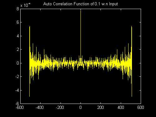
figure
plot(index_expanded,r_xx_w_2_expanded)
title(['Auto Correlation Function of 0.1 w.n Input'])
%************************************************************
|